ViewCube
The aim of ViewCube is to remain lightweight and independent of the operating system. Currently, there are no buttons or interface, only two plotting windows. All interactions are performed using the mouse and keyboard. This tutorial will cover the different options and their corresponding keys. Additionally, there is a Cheat Sheet containing a table with each key and its associated action.
There are plans to significantly improve ViewCube by switching to a faster plotting library and introducing a menu interface. However, this is still under development.
Basic call
To visualize a data cube, simply provide the name of the FITS file in the command line
ViewCube datacube.fits
If the installation was successful, you should be able to call ViewCube from any directory.
Command line options
To learn about the command line options and arguments for ViewCube, simply type:
ViewCube -h
usage: ViewCube [-h] [--data DATA] [--error ERROR] [--flag FLAG] [--header HEADER] [-a A] [-b B] [-c C]
                   [-e] [-f] [-fo FO] [-fc FC] [-i] [-k] [-m] [-p P] [-s S] [-y Y] [-v] [-w W]
                   [--config-file] [name ...]

positional arguments:
  name             FITS file (default: None)

options:
  -h, --help       show this help message and exit
  --data DATA      DATA extension (default: None)
  --error ERROR    ERROR extension (default: None)
  --flag FLAG      FLAG/MASK extension (default: None)
  --header HEADER  HEADER extension (default: 0)
  -a A             Angle to rotate the position table (only RSS) (default: None)
  -b B             Matplotlib backend. Use 'TkAgg' if using PyRAF for interactive fitting. Available
                   backends: GTK3Agg | GTK3Cairo | GTK4Agg | GTK4Cairo | MacOSX | nbAgg | QtAgg | QtCairo |
                   Qt5Agg | Qt5Cairo | TkAgg | TkCairo | WebAgg | WX | WXAgg | WXCairo (default: QtAgg)
  -c C             FITS file for comparison (default: None)
  -e               Position table is in RSS and -p indicates the extension (string or int) (default: False)
  -f               Do NOT apply sensitivity curve (if HDU is available) (default: True)
  -fo FO           Multiplicative factor for original file (default: 1.0)
  -fc FC           Multiplicative factor for comparison file (default: 1.0)
  -i               Conversion from IVAR to error (default: False)
  -k               Use X,Y instead of sky coords for computing fiber distance (default: True)
  -m               Do NOT use masked arrays for flagged values (default: True)
  -p P             External position table for RSS Viewer (default: None)
  -s S             Spectral dimension (default: None)
  -y Y             Plot style, separated by comma: 'dark_background, seaborn-ticks' (default: None)
  -w W             HDU number extension for the wavelength array (default: None)
  --config-file    Write config file (default: False)
Using ViewCube
When a properly formatted FITS datacube is provided, ViewCube opens two windows: the spaxel viewer and the spectral viewer. Depending on the backend used, these titles will be assigned to the windows. If not, “Figure 1” will appear in place of the spaxel viewer, and “Figure 2” will be used for the spectral viewer.
Spaxel Window
Spectral Window
Each window has its own set of actions, which can be triggered by mouse movements, clicks,
or specific key presses. Some keys, such as q for quitting, are shared between windows,
while others are unique to each window and only function when that window is active.
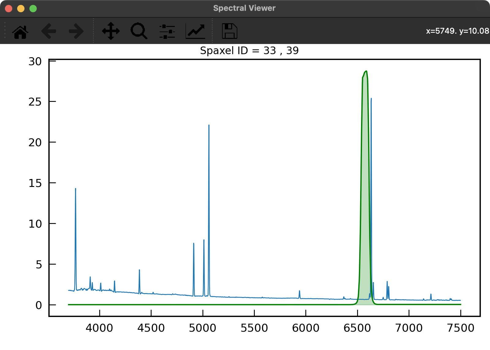
Spectral Window
In the spectral window, the spectrum of each spaxel is displayed when the mouse hovers over the 2D map.
The x-axis units are in Angstroms by default, while the y-axis units in the spectral window are shown in the native units of the datacube.
Setting Axis Range
By default, the spectral window in ViewCube adjusts the x-axis to the full wavelength
range of the plotted spectrum and the y-axis to the full flux. If you want to zoom in
on a specific wavelength or flux range, you can do so by pressing the l key to set
the wavelength range and Y (capital) to set the flux (y-axis).
Enter two values separated by a comma in the command line (e.g., 6550,6700 for the
x-axis). To set one of the extremes as the default, simply input None for that
value (e.g., None,4500).
To reset to the full range, enter None, None.
Toggling the Error Spectrum
If the FITS file contains an error datacube in one HDU (you can specify this as an argument when opening a datacube), you can toggle the error vector, which will appear as uncertainty (gray) bars over the spectrum.
Toggle the error spectrum (if available) by pressing the e key.
Setting Redshift
To facilitate the visualization of spectra, you can shift the wavelength of the spectra
to the rest frame or to any velocity. First, ViewCube will attempt to read a keyword
in the main header called MED_VEL, which represents the recession velocity of the
object in km/s. By pressing the z key, the spectrum will shift in wavelength by the
amount specified in the velocity.
Shift the wavelength using the z key.
Be sure to press the z key when the spectral window is active; otherwise, if the
spaxel window is active, you will activate the ZSCALE mode
(see below Color maps section).
If the keyword is not present in the header, you can introduce (or override) the value
by pressing the k key and entering the desired value in km/s in the command line.
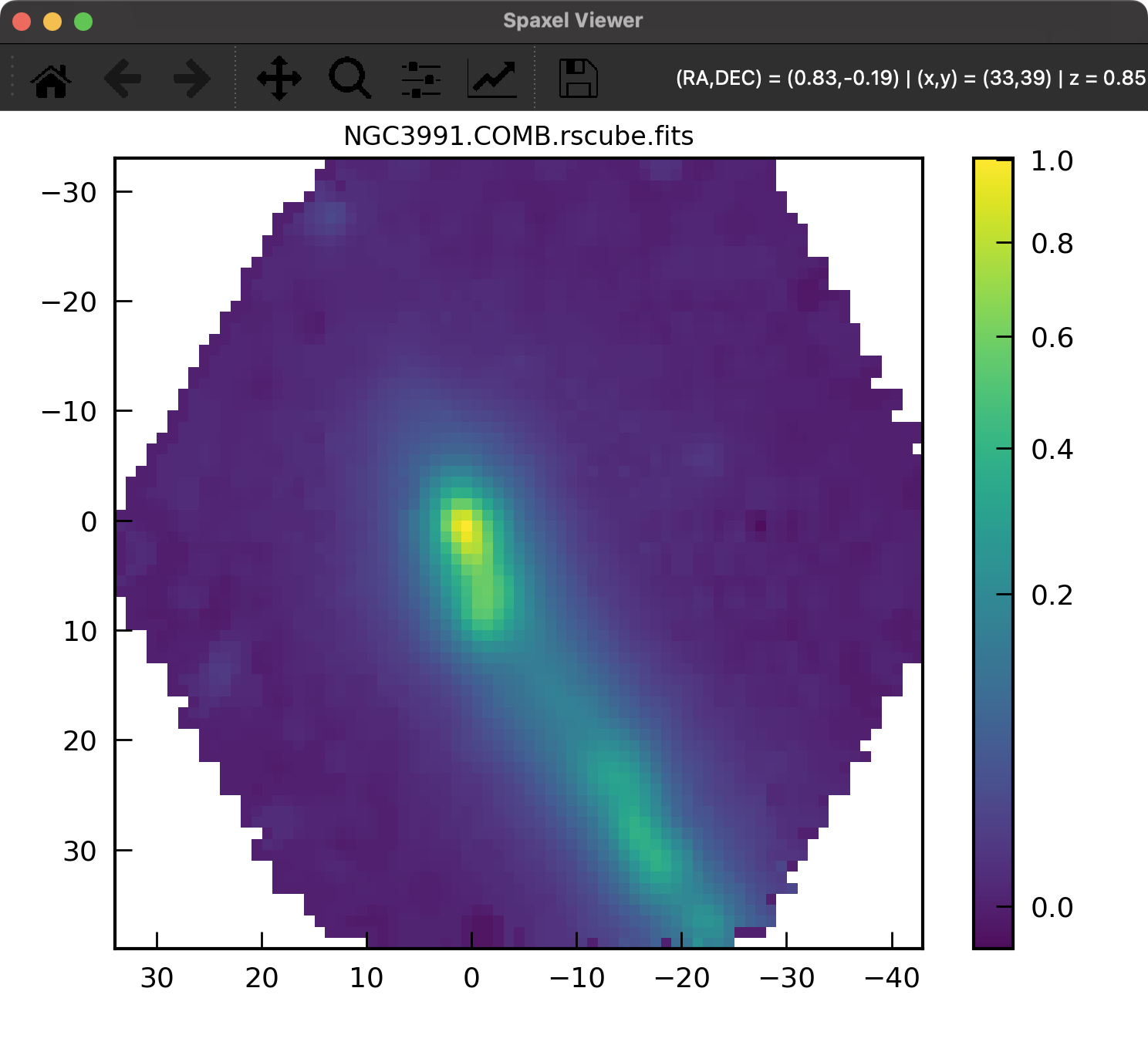
Spaxel Window
The spaxel window displays a 2D map of the datacube, convolved in the spectral direction using a specific filter, which is represented as a green shaded area in the spectral window. If no filters are available, a default box filter is applied.
The axes of the spaxel window are displayed in the units specified in the FITS header, if
available. Viewcube attempts to use arcseconds for the axes if unit information is
provided; otherwise, it defaults to pixel units. The reference pixel is derived from the
CRPIX1 and CRPIX2 values in the header, with offsets calculated in either
arcseconds or pixels, which are then shown in the x and y tick labels.
Move the mouse over the 2D image of your object, and the spectral window will display the corresponding spectra for that specific spaxel.
The spaxel coordinates (in pixel units) will appear both in the spaxel viewer, using matplotlib’s built-in mouse position information in the upper right corner, and as the figure title in the spectral window.
To pause and freeze the spectra at a specific spaxel, press s. To resume the
spaxel-spectra interactive plotting, press s again.
Filter configuration
To convolve the cube with a specific filter or set of filters, a directory containing the filter files must be specified in the ViewCubeRF configuration file. This directory should contain only ASCII files, with each file representing one filter. ViewCube will read all files in the directory, making them available for selection in a cyclical manner.
Each filter file must include at least two columns: the first column should list the wavelength in Angstroms, and the second column should specify the filter’s throughput at each corresponding wavelength. Any additional columns will be ignored.
#  Wavelength  Transmission
      5200.00       0.00000
      5250.00       0.01000
      5300.00       0.02000
      5350.00       0.04000
      5400.00       0.06000
      5450.00       0.11000
      5500.00       0.18000
        ...           ...
      9300.00       0.01000
      9350.00       0.01000
      9400.00       0.01000
      9450.00       0.01000
      9500.00       0.00000
To change the filter, press t to move forward through the filter cycle or T to go backward.
These are some of the keys that work in both the spaxel and spectra windows. You
You will notice how the green-filled area in the spectral window changes across the displayed spectra, and how the 2D image in the spaxel window adjusts accordingly. Keep in mind that some filters may fall outside the datacube’s spectral coverage and will not appear in the spectral window.
Changing the filter using the t (forward) or T (backward) keys.
To specify the filter directory for ViewCube, open the .viewcuberc configuration file,
uncomment the dfilter variable, and provide the ABSOLUTE path inside quotation marks:
dfilter: "/absolute/path/to/filters/directory/"
You can also set the default filter for ViewCube by editing the .viewcuberc config file
and defining the name of the filter file:
default_filter : "Halpha_KPNO-NOAO.txt"
Drag-and-Drop Filter Feature
You can modify the 2D image map in the spaxel window by dragging and dropping the filter to a different position along the spectral axis. To do this, click inside the green filled area, hold down the mouse button, drag the filter to the desired location, and release the button. The spaxel window will update accordingly.
Drag and drop the filter to reapply the convolution to the datacube.
A filter wavelength range may be outside the actual spectrum wavelength range, and
thus, it might not appear in the plotting window. You can move and center the filter
to the central wavelength range of your plotting window by pressing the a key.
Continuum removal
ViewCube includes a simple algorithm to remove the continuum from the filter. You can
activate continuum removal by pressing the c key, which will update the spaxel
window map. This feature is useful for quickly visualizing HII regions when using a
narrow filter, for instance. Press the key again to return to the standard view.
Remove continuum by pressing c; press again to restore the original view.
Color maps
All color maps for the 2D plot are available from the Matplotlib library. You can change the
color map in the spaxel window by pressing the + key (to move forward) or the - key
(to move backward).
To view the available color maps, press m, and they will appear in the command line window.
Press ENTER to exit the color map selection, or type the name of the desired color map to apply it.
You can also invert the color map by pressing the i key.
There is also an option to adjust the stretching and normalization of the color map. Press the
z key to toggle between ZSCALE normalization (as used in DS9) and the default setting.
To modify the stretching, use the number keys from 1 to 5:
Key |
Stretching |
|---|---|
1 |
Linear |
2 |
Log |
3 |
Sqrt |
4 |
Power |
5 |
Asinh |
You can also dynamically adjust the max and min values to optimize the dynamic range. To do this, press and hold the right mouse button on the spaxel window (2D map), then move the cursor up-left or left-right, similar to the behavior in DS9.
Change colormap dynamic range (by pressing and holding the right mouse button)
Alternatively, you can manually set the min/max values for the color map by pressing the
v key and entering the values in the command line, separated by a comma:
For example: 5,20
Use None if you want to modify only one of the values, such as:
-1, None
Spaxel selection
Users can select multiple spaxels for easier comparison. In the spaxel window, click the left mouse button to select a specific spaxel. Alternatively, users can hold the mouse button and move the cursor over the 2D map to select multiple spaxels simultaneously.
Spaxel selection (by pressing the left mouse button)
If a spaxel has been selected erroneously or is no longer needed, press the d key and
hover the mouse over the spaxel in question. While holding down the ‘d’ key, the mouse will
delete selected spaxels as you hover over them. Release the d key to return to
default mode.
Deleting selected spaxels by pressing the d key
If you want to delete all selected spaxels, simply click the * key.
Comparing spectra
To view the spectra of selected spaxels, navigate to the spectral window and click the
right mouse button. Three main plotting options are available: the first displays the
individual spectra; the second combines the individual spectra with the integrated
spectrum, which is the coadd of all spaxels; and the third shows only the integrated
spectrum. You can cycle through these options by clicking the right mouse button.
To identify which spectrum in the spectral window corresponds to a specific spaxel, click on the desired spectrum. A colored rectangle (matching the color of the spectrum line) will be drawn around the corresponding spaxel in the spaxel window. Additionally, a label with the spaxel coordinates will appear in the figure title of the spectral window.
Saving spectra
Once you have selected several spaxels, you can choose to save either the integrated spectrum or the individual spectra. To save the data to a file, press the “S” key (capital letter). You will be prompted to enter a root name for the file in the command line. If saving as an ASCII file, the “.txt” suffix will be automatically appended (e.g., “spectrum.txt” if “spectrum” is the root name). If you choose to save the spectra from individual spaxels in separate files, the file names will also include the coordinates of each spaxel (e.g., “spectrum_33_55.txt” for a spaxel at coordinates 33,55).
Window manager
In the current version of ViewCube, the only window with “buttons” is the window manager, which can be activated by pressing the “W” key (this works if either of the two main windows is active).
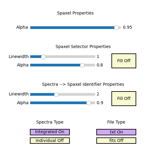
Window Manager
In the window manager, you can select the file format for saving the integrated and individual spectra (either ASCII, FITS, or both). Additionally, you can choose whether to save the integrated spectra, individual spectra, or both.
It is possible to also change the spaxel selec
Fitting Package Options
To facilitate a more in-depth analysis of a particular spectrum, the current version of ViewCube includes an interactive fitting mode that leverages the capabilities of other programs. It can interact with external packages, specifically PySpecKit and Pyraf’s splot.
Press the i key to choose and cycle between the Pyraf and
PySpecKit selections.
Ensure that these packages are installed to use them. If only one package is
installed, that will be the default mode, and pressing i will not change anything
since there is nothing to cycle through.
Once you have selected the package you want to use (as indicated in the command line),
select a spaxel (see the section on Spaxel Selection above).
Then, press the x key, and a new window will open with the spectrum of the selected
package displayed in that program.
Visualizing Raw-Stacked Spectra (RSS) files
In its ViewRSS mode, ViewCube can also read Raw-Stacked Spectra (RSS), which is particularly useful for inspecting individual dithers, for example. To enable this, ViewCube requires information about the fiber size and configuration. This data can be automatically retrieved from the FITS file if there is an HDU containing a table with the fiber details, or it can be provided through an external ASCII file.
For example, if you have an RSS FITS file with the following
structure (as shown by fitsinfo):
Filename: NGC2906_p1.sobj.fits
No.    Name      Ver    Type      Cards   Dimensions   Format
  0  PRIMARY       1 PrimaryHDU     148   (1877, 331)   float32
  1  ERROR         1 ImageHDU         8   (1877, 331)   float32
  2  BADPIX        1 ImageHDU         8   (1877, 331)   uint8
  3  POSTABLE      1 BinTableHDU     23   331R x 4C   [E, E, I, 3A]
You can inform ViewCube that the position table is located within the FITS file by using
the -e flag, along with the -p option to specify the HDU number extension:
ViewCube -e -p 3 NGC2906_p1.sobj.fits
Alternatively, if you have a fiber position table in an ASCII file, you can specify it using
the -p option:
ViewCube -p position_table.txt rss_file.fits
The plotting and interactive capabilities of ViewRSS are similar to those of ViewCube. You can select and compare fibers in the same way you would with spaxels in a datacube.
ViewRSS